I can't color my pie chart based on the conditional format.
Resolved
Based on the doc, there must be the option to enable the existing conditional format in the chart series.
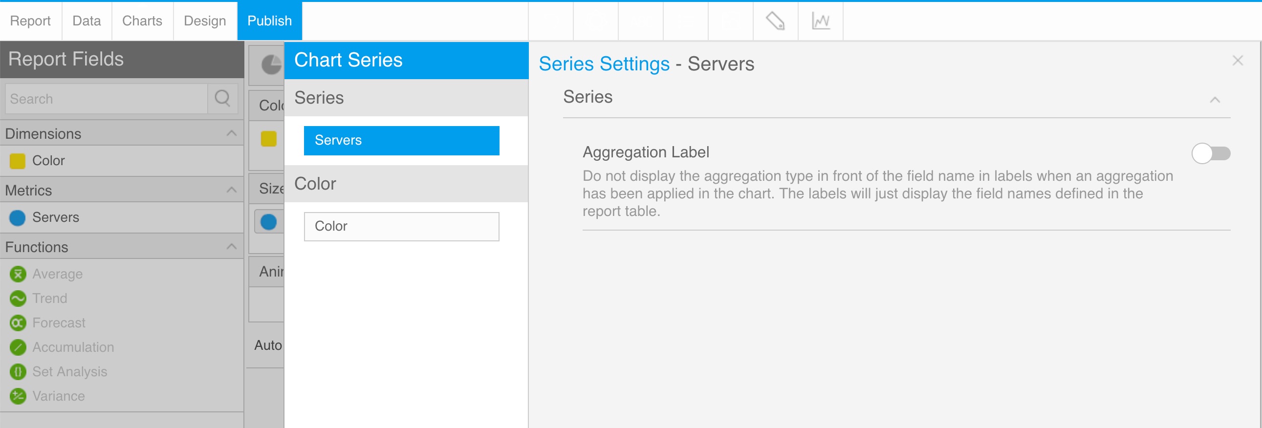
I don't have that option, only the "Aggregation Label", but not what is needed to do that.
What I'm doing wrong here?
 The same problem
Hi Matthias,
Thanks for reaching out. What doc are you referring to here?
I believe what you may be looking for would be covered in the following Idea item: Advanced Conditional Formatting on a Chart.
Can you please read through this Idea and let me know if this appears to be what you're looking for? If so, feel free to vote on this Idea, which could aid in this being considered for future implementation. Either way, please let me know.
Regards,
Mike
Hi Matthias,
Thanks for your response. Not all Series options are available for each chart type. As you can see, if I set up Conditional Formatting at the chart level and do an Auto-Chart, which in this case is a Horizontal Bar Chart, I have the option:
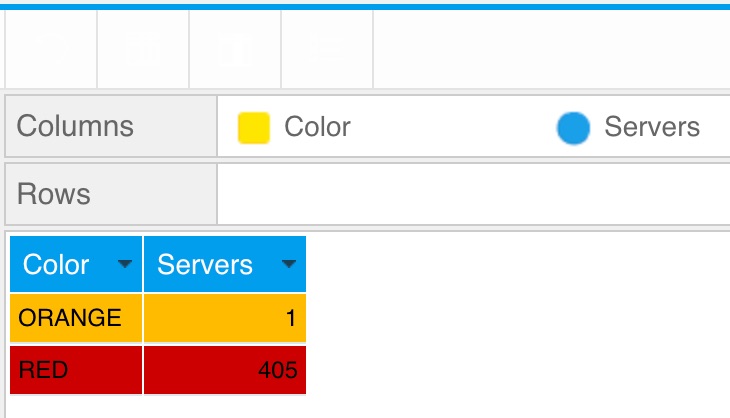
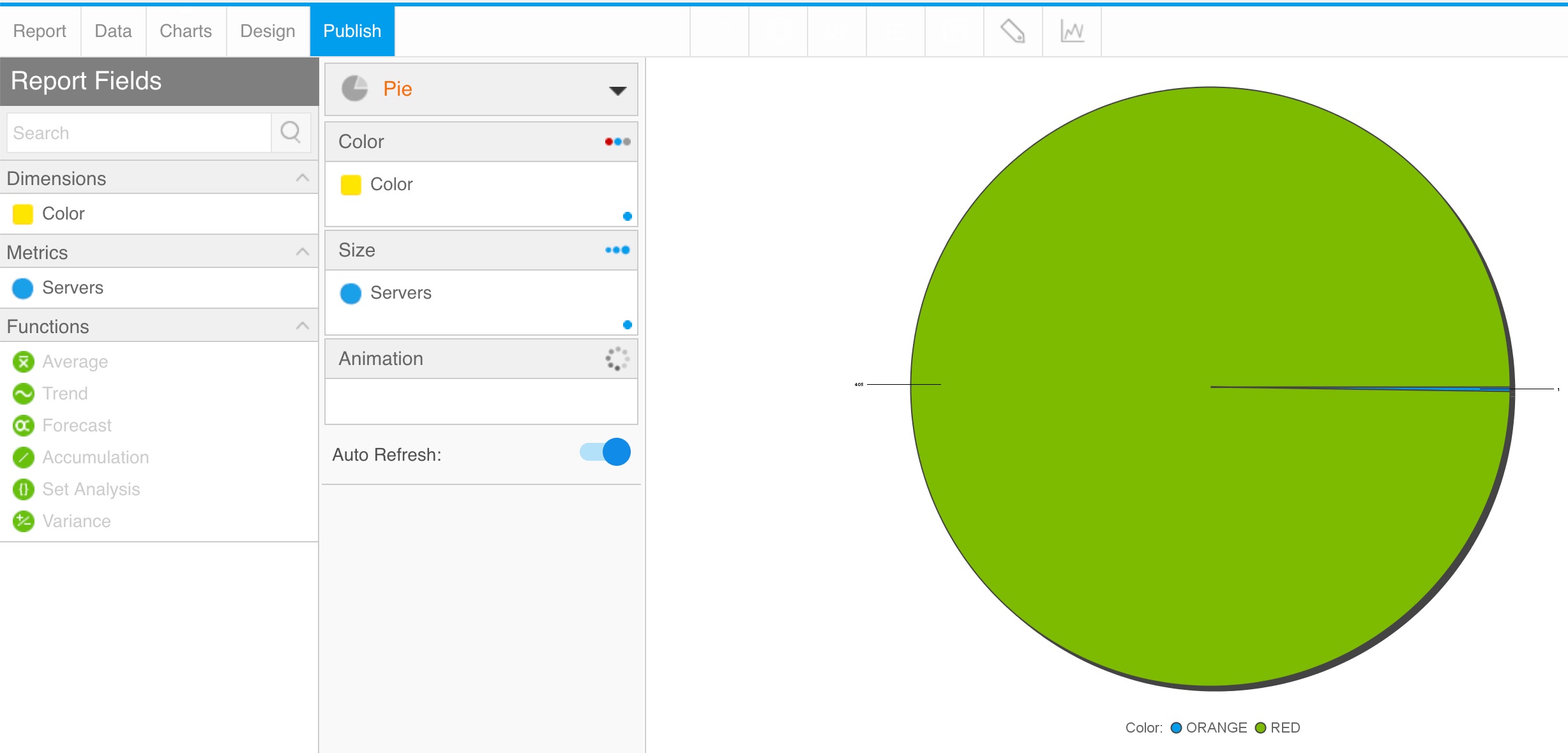
However, this makes sense, because in the Pie Chart you follow the color of the Dimension, which is not the Series data. In your case this is the 'Color' Dimension, while your Series is the 'Servers' Metric.
Using my example above, what I need to do is apply conditional formatting on my Dimension data ('Athlete Region'), but in order to make the formatting follow results from another column, in this case the 'Sum Invoiced Amount' values, I have to use the Advanced Conditional Formatting option, setting it up like so:
This is where the issue regarding the referenced Advanced Conditional Formatting on a Chart Idea comes in, since as you can see, there's no option to choose Advanced Conditional Formatting:
As a workaround, you can use Basic Conditional Formatting, manually making them match values from another column, like so:
As you can see, I now have the option:
Hopefully this clears things up a bit. Please let me know if you have any questions on this.
Regards,
Mike
Hi Matthias,
Thanks for your response. Not all Series options are available for each chart type. As you can see, if I set up Conditional Formatting at the chart level and do an Auto-Chart, which in this case is a Horizontal Bar Chart, I have the option:
However, this makes sense, because in the Pie Chart you follow the color of the Dimension, which is not the Series data. In your case this is the 'Color' Dimension, while your Series is the 'Servers' Metric.
Using my example above, what I need to do is apply conditional formatting on my Dimension data ('Athlete Region'), but in order to make the formatting follow results from another column, in this case the 'Sum Invoiced Amount' values, I have to use the Advanced Conditional Formatting option, setting it up like so:
This is where the issue regarding the referenced Advanced Conditional Formatting on a Chart Idea comes in, since as you can see, there's no option to choose Advanced Conditional Formatting:
As a workaround, you can use Basic Conditional Formatting, manually making them match values from another column, like so:
As you can see, I now have the option:
Hopefully this clears things up a bit. Please let me know if you have any questions on this.
Regards,
Mike
Hi Mike,
sorry for my late reply I was traveling and want to take the time now to thank you for your support.
Changing the conditional formatting to basic solved my issue and I could colorize my chart as defined.
Thank you,
Matthias
Hi Mike,
sorry for my late reply I was traveling and want to take the time now to thank you for your support.
Changing the conditional formatting to basic solved my issue and I could colorize my chart as defined.
Thank you,
Matthias
Hi Matthias,
Great! Thanks for confirming. I'll go ahead and close this case out then, but please don't hesitate to reach back out with any other questions or concerns on this or anything else.
Regards,
Mike
Hi Matthias,
Great! Thanks for confirming. I'll go ahead and close this case out then, but please don't hesitate to reach back out with any other questions or concerns on this or anything else.
Regards,
Mike
Replies have been locked on this page!